| Source | Program | Pull | Window | Tidy artefact |
|---|---|---|---|---|
| BLS CES | Current Employment Statistics, national, seasonally adjusted, all employees | BLS Public Data API v2 | 2010-01 → 2026-03 | data/processed/bls_ces_national_monthly_long.csv, ..._indexed_long.csv |
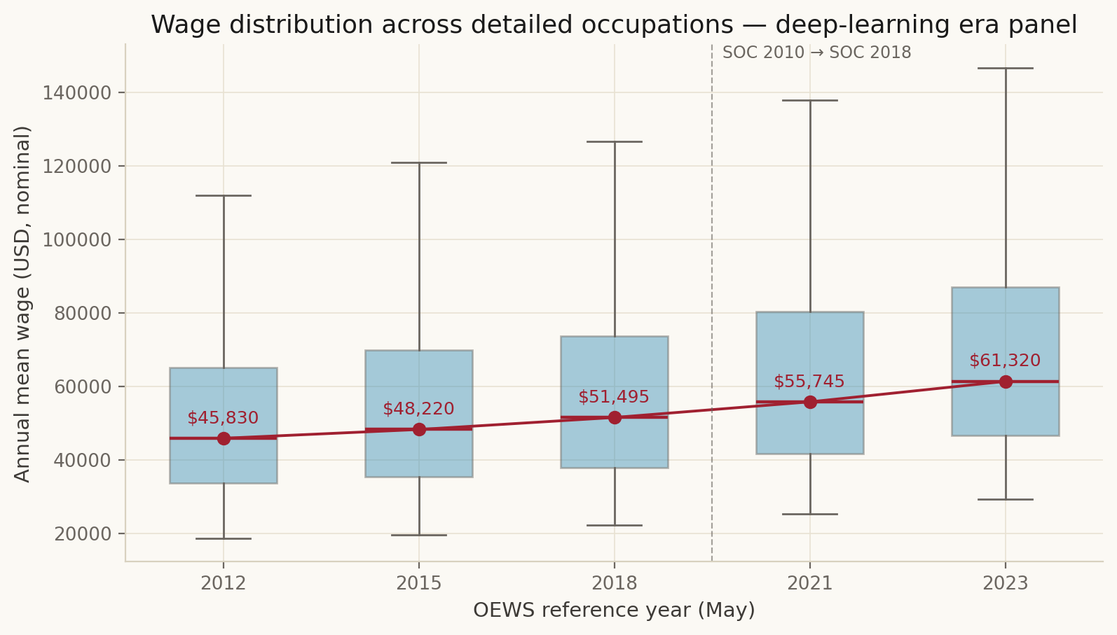
| BLS OEWS | Occupational Employment and Wage Statistics, national, detailed SOC | XLSX bulk download (2012, 2015, 2018, 2021, 2023) | 2012 → 2023 | data/processed/oews_national_panel_long.csv |
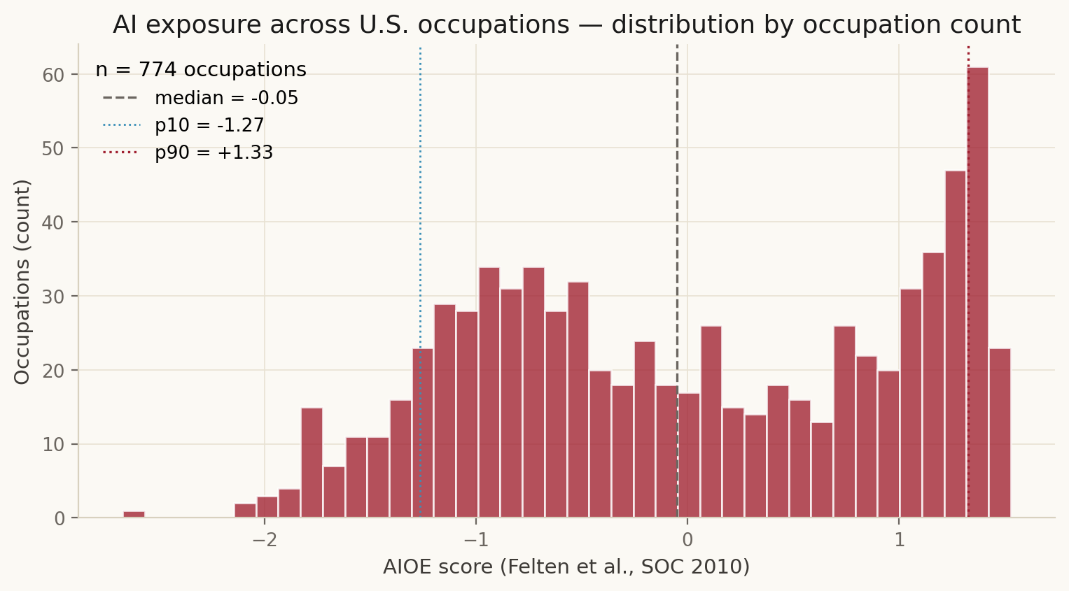
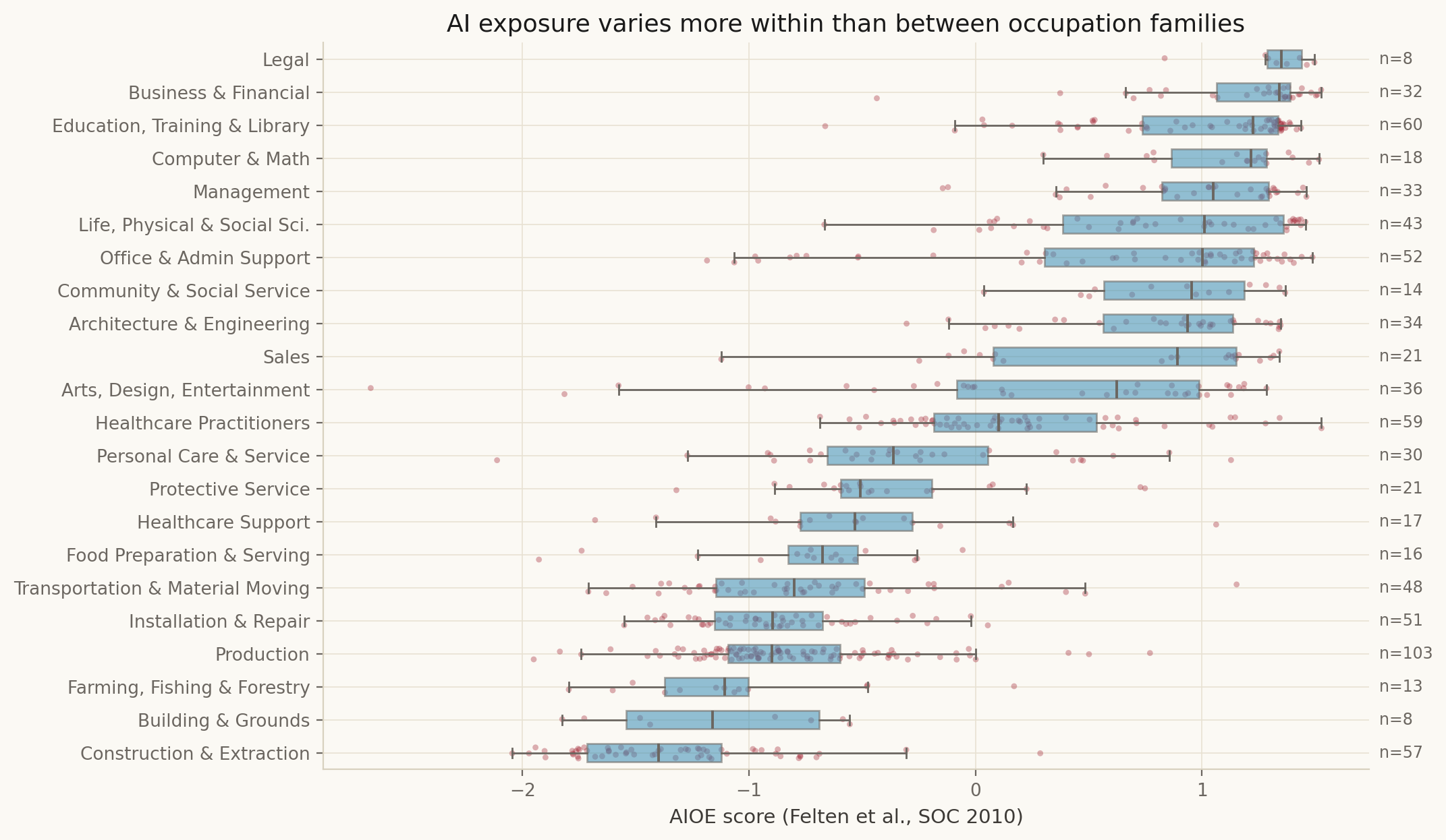
| Felten et al. | AI Occupational Exposure (AIOE), SOC 2010 | Appendix XLSX | static (2018 release) | data/processed/aioe_soc_2010.csv (n = 774) |
All retrieval, cleaning and tidying scripts live under scripts/. Snapshots of basic stats are in data/meta/DATA_SNAPSHOT.md, data/meta/OEWS_PANEL_SNAPSHOT.md, and data/meta/data_diary.md.
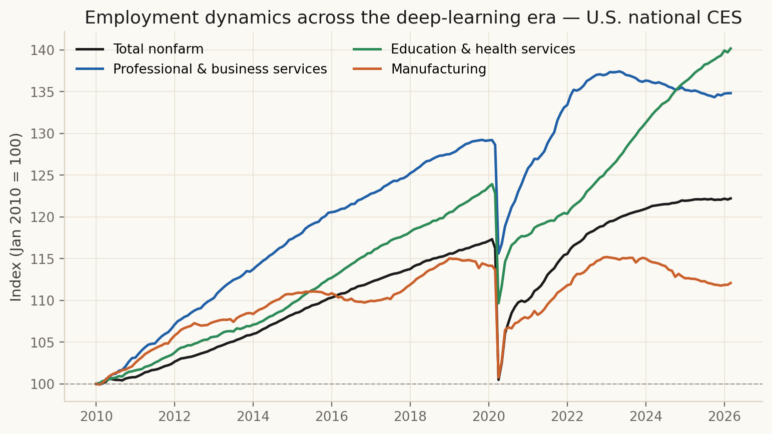
Let (E_{s,t}) be employment for series (s) at month (t), and let (t^*) be the earliest month in which all series in the panel have a non-missing observation. The indexed value is
[ _{s,t} = 100 , . ]
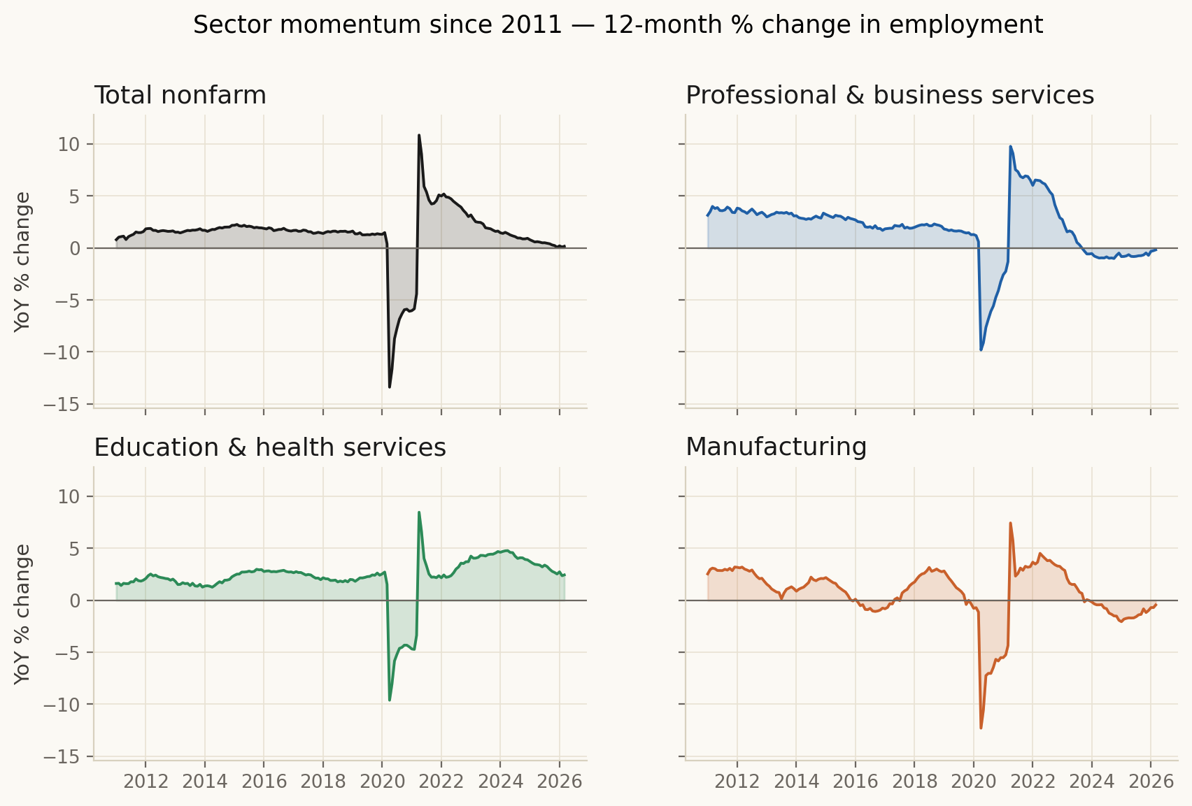
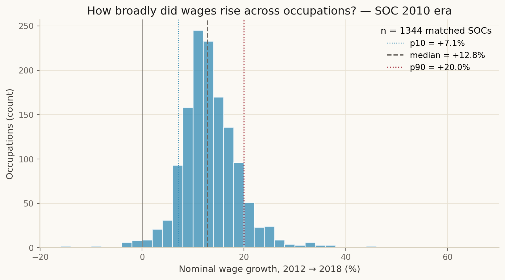
Year-over-year percent change (Figure 02) uses raw CES levels within each series:
[ _{s,t} = , . ]
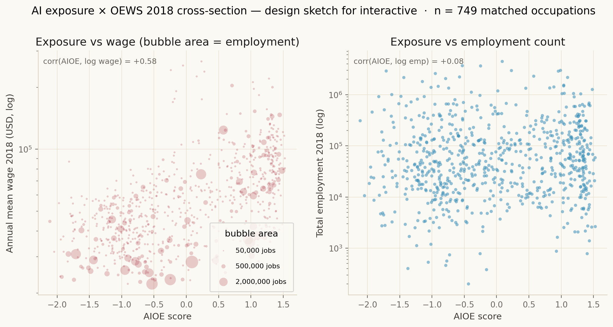
Felten et al. publish AIOE on SOC 2010 (n = 774 detailed occupations). OEWS uses SOC 2010 through 2018 and SOC 2018 from 2019 onward. The vintage flip breaks naive year-over-year SOC joins past 2018, so we only merge AIOE with OEWS on SOC 2010 records (2012, 2015, 2018) for the cross-sectional Figure 08, and we restrict the longitudinal thesis-test (Figure 09) to occupations whose SOC code persists across both vintages.
For each AIOE quartile (Q) and year (y) we compute
[ r_{Q,y} = ]
and report (r_Q = r_{Q,2023} - r_{Q,2012}). A widening (r_{Q4}) is the predicted signature of the “AI throne” thesis — top-end pulling away from the median fastest where AI exposure is highest. We observe (r_{Q4} ) through 2023.
Top-coding caveat. OEWS publishes p90 with a BLS ceiling (≈ $208 k in 2018, raised to ≈ $239 k by 2023). Wages above the ceiling are reported at the ceiling. This makes the test conservative: it suppresses signal at the top of high-AIOE distributions. Any signal that survives top-coding is real; absence of signal does not foreclose the thesis above the ceiling, where post-LLM compensation effects are most likely to land.
OEWS suppresses cells with insufficient sample. Suppressions appear as NaN in the wage columns and are dropped from quantile computations. Counts of dropped cells per anchor year are recorded in data/meta/OEWS_PANEL_SNAPSHOT.md.
The thesis the page engages is fundamentally about capital share and post-LLM dynamics. The page is honest that BLS occupation-level data through 2023 cannot test most of it. The Coda watchlist names the data sources that can: BEA factor-share series, top-1 % income panels (Piketty / Saez / Zucman), JOLTS by occupation × industry post-2022, post-2024 OEWS releases, and firm-level AI-adoption surveys.
This project used AI assistance for code, layout, design, and copy editing. The narrative — topic, thesis, four-act structure, per-figure editorial calls, all body prose — was authored and finalised by the human author. AI was treated as a paired contributor whose outputs were reviewed and edited; AI was not the author of the narrative.
| Tool | Role |
|---|---|
| Cursor (Claude Sonnet / Opus) | Coding agent: data-pipeline scripts, Plotly/matplotlib chart code, Quarto wiring, layout debugging, screenshot inspection. |
| Claude Design (Anthropic Sonnet, “Design” mode) | Single-pass production of the visual design system (palette, typography ramp, motion budget, component CSS, Plotly/Observable themes). |
ydata-profiling (no AI) |
Deterministic profiling reports for QA — not LLM-driven; included here for completeness because it sits in the same pipeline. |
Two prompts shaped the project; both are committed in the repository so the audit trail is reproducible.
Claude Design production prompt. A single brief that locked the editorial spine, the data the design system could read, the deliverable list (interactive charts, linked view, infographic, optional hero), and the voice discipline (“labor-economics vocabulary, not partisan triggers”). The full text is at notes/CLAUDE_DESIGN_PROMPT.md. Excerpt:
You are a senior data-visualization designer for a public-interest narrative web feature on AI exposure and the U.S. labor market, January 2010 → present. The data pipeline is built (BLS CES + OEWS + Felten et al. AIOE); the editorial story is locked from completed EDA; eight matplotlib drafts are already triaged. Your job is to produce the production layer: interactive charts, one linked view, one closing infographic, and an optional hero — to a Reuters/Pudding-adjacent quality bar.
[…] Use labor-economics vocabulary, not partisan triggers — say “capital concentration / labor share / substitution vs augmentation,” not “ultra-rich / throne / cyberpunk.” The hook can speak to the worry; the chart language must remain professional.
EDA / discovery discipline. AI agents were instructed to operate on the data layer by discovery from artefacts only (CSV, profiles, snapshots), never from narrative defaults: do not treat PROJECT_PLAN.md, chat hypotheses, or sector narratives as facts until they appear in data artifacts; treat the pipeline as a discovery loop — data/processed/ tables, data/meta/DATA_SNAPSHOT.md, and profile_dataset.py outputs are the source of truth for numbers.
The Claude Design pass returned a self-contained design-system bundle. The following files were taken from that bundle and are in production on the site:
| File in repo | Source | Role |
|---|---|---|
narrative_site/_design/colors_and_type.css |
Claude Design output | CSS variables (palette, type ramp, spacing). Loaded by _quarto.yml. |
narrative_site/_design/quarto-overrides.css |
Claude Design output | Neutralises Quarto’s bootstrap defaults so design tokens win. |
narrative_site/_design/narrative-components.css |
Hand-translated from Claude Design’s JSX reference | Editorial header, hero, act sections, figure frames, watch-grid. |
narrative_site/_design/ui_kits/figures/plotly_theme.py |
Claude Design output | Python Plotly theme (apply_theme, COLORS, HTML_CONFIG) used by all 9 interactive figures via the shim scripts/figs/_plotly.py. |
narrative_site/_design/ui_kits/figures/plotly_theme.js, observable_theme.js |
Claude Design output | JS-side themes for any direct Plotly.js / Observable Plot use. |
narrative_site/_design/assets/icons/lucide/*.svg |
Lucide icon set, selected by Claude Design | Coda watch-grid iconography. |
narrative_site/_design/INTEGRATION.md, README.md, SKILL.md |
Claude Design output | Wiring documentation kept verbatim. |
Every Plotly chart in the page (figs/fig_0{1..9}_interactive.html) calls apply_theme() from this bundle. The matplotlib statics in scripts/figs/_common.py were retoned by hand to the same tokens (matplotlib has no way to read CSS; the Python palette is a deliberate copy).
fig_0{1..9}_interactive.py), the Quarto raw-HTML scaffold for index.qmd, and the matplotlib _common.py palette wiring.iframe heights.narrative-components.css).Every number quoted in the page (correlations, percent changes, percentile ratios, occupation counts) is computed from the committed processed CSVs in data/processed/ by the committed scripts in scripts/. AI agents were instructed by the EDA skill above never to invent statistics. If a number appears in the article, it is reproducible from a script in this repo.
The eight matplotlib counterparts to the interactive figures on the main page. These are the print-ready, no-interaction reads of the same data. Each is generated by the matching scripts/figs/fig_NN_*.py script and shares the design-system palette via _common.py.
SVG vector versions of all eight are also committed alongside the PNGs (figs/fig_NN_*.svg).